A psychometric function is a plot of detectability against the intensity of the stimulus. There is a range of intensities over which the subject will sometimes report a signal and sometimes will not. The measure of detectability used in a psychometric function can either be simple, such as the percentage of detections or a more calculated measure, such as d'. Green and Swets (1974) discuss the measure of d' in terms of signal detection theory. Welford (1968) describes the mapping between percentage correct and d' (which assumes the listener has no bias). In practice, it is not necessary to calculate mappings between a percentage measure and d' as tables exist that allow d' to be read off given the number of choices (e.g. 2 or 3 alternatives) and the proportion correct. In the context of the detection time model, it is reasonable to assume that if detection time increases, then the proportion of correct responses will rise according to some undetermined monotonic function. The modelling presented in chapter 6 suggested that the slopes of the psychometric functions should be steeper for the correlated condition than for the uncorrelated condition. To check this prediction it was decided to experimentally measure psychometric functions for conditions which were similar to those presented to the model (based on experiment 3). Only a very small subset of the conditions in experiment 3 was used due to the time consuming nature of deriving psychometric functions. It should be noted that each of the previous measures corresponds to one point on the psychometric function. A three-down, one-up procedure (as used in all the previous experiments) tracks the 79.4% correct point on the psychometric function (Levitt, 1971). With a three-alternative force choice procedure, this corresponds to a d' of roughly 1.6.
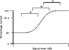
The task in experiment 5 was to detect a 20-Hz wide band of noise centred at 1500 Hz. Two masking bands (also 20 Hz wide) were centred at 900 and 2100 Hz. The masking bands had a spectrum level of 65 dB SPL which corresponds to each having 78 dB SPL overall level. The masking bands were always correlated with each other. The signal could be either correlated or uncorrelated with the masking bands. Five signal levels were presented in a cyclic order decreasing in intensity as described by Moore and Sek (1992). This gives the subject a reminder of what the signal sounds like every 5 observations. If each signal level is presented independently for a whole block of observations, it is very easy for the subject to lose track of the signal especially at low signal levels. The results may be different for the two techniques, but it was felt that the cyclic technique provides a more accurate measurement of the psychometric function. The signal levels were equally spaced in dB and were chosen on the basis of per-subject piloting. Choosing the correct range of signal levels is very important. This is illustrated in figure 7.1.

Figure 7.1. An idealised psychometric function for a 3-alternative forced choice experiment. A number of possible ranges are shown. Of the 3 shown, range B will be less prone to floor and ceiling effects.
Figure 7.1 shows an idealised psychometric function and the classic 'S' form. A number of signal level ranges are shown. In the analysis of psychometric functions, points from the very extremes of the functions should be disregarded. As the curve approaches the floor and ceiling, the slope flattens and thus any analysis that includes points from these sections of the curve will be inaccurate. As the measurement of psychometric functions can be very time consuming, signal levels should be concentrated in region B.
The conditions used in experiment 5 correspond to the C600 and U600 conditions from experiment 3. The threshold measured in the earlier experiment was therefore used as a guide for choosing the signal levels. The thresholds correspond to the 79.4% point on the psychometric function (Levitt, 1971) as a three down, one up procedure was used in experiment 3. A 3-alternative forced choice (3AFC) means that chance is at 33% correct. It is therefore quite easy to determine suitable signal levels with the minimum of piloting. The threshold to the nearest dB was chosen as the central signal level and two levels on either side were chosen. Brief pilots were run to determine the spacing and the exact levels to be used.
The stimuli were derived from those used in experiment 3. The signal was presented at random in one of three observation intervals which were marked by lights on the response box. The intervals were separated by 200 ms. The two masking bands were simultaneously gated with the signal. Signal timing was controlled by a Texas Instruments 990/4 computer. Each gate consisted of two analogue multipliers (AD534L) connected in series. The gating voltages were derived from 12-bit digital-to-analogue converters. The signal level was controlled by a Charybdis model D programmable attenuator.
The signal was presented at one of five signal levels which were cyclically chosen (highest first) from the levels specified (e.g. 40, 38, 36, 34, 32, 40, 38...). In each run, every signal level was presented ten times (i.e. fifty observations per run). For each subject, 20 complete runs were obtained so that there were 200 observations per signal level.
Three subjects participated, all with absolute thresholds less than 10 dB HL at all audiometric frequencies. All subjects had previously completed earlier experiments.
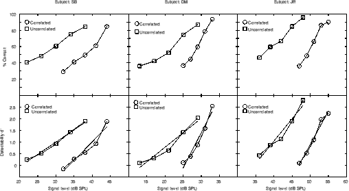
Given the percentage correct and the number of alternative choices, it is possible to use tables to convert the percentage values to d', the measure of detectability. Figure 7.2 shows the results for all subjects plotted both as percent correct and as d'.

Figure 7.2. The results of all three subjects in experiment 5. Each column represents a different subject.The top row shows the percentage correct results. The bottom rows shows the results converted to d'. Linear regression lines fitted to the d' values are shown.
The bottom row in figure 7.2 shows d' plotted against the signal level. Note that the signal levels were different for each subject. The slopes of the psychometric function clearly differ between the correlated and uncorrelated conditions. Lines of best fit were calculated by linear regression for the d' values. The results are shown in table 7.i.
![]()
Table 7.i. The slopes of the psychometric functions in figure 7.2
The calculated slopes are clearly very different between the two conditions. A t-test was performed on the slopes of the psychometric functions (Snedecor and Cochran, 1967). The t(8) values were significant for all subjects at the p=0.05 level with the difference for subject DM being significant at p<0.001 (t(8)=2.21 (SB), 5.11 (DM), 2.34 (JR)). The gradient of the psychometric function for the correlated condition is roughly twice that for the uncorrelated condition. Figure 6.7 shows that the model described previously predicts that the psychometric functions will differ in slope. There is little point in calculating the slopes of the lines in figure 6.7 and comparing them with the values in table 7.i as the function that relates detection time to detectability is not known.
The model that predicted the observed difference in the slopes of the psychometric functions is based on a purely within-channel mechanism, as the output is dependent upon only one simulated filter centred on the signal frequency. As described in chapter 6, the slopes of the psychometric functions would be expected to be sharper in the correlated condition if a within-channel mechanism is responsible for the CDD. There is no obvious reason why such a difference should exist with an across-channel mechanism. Moore et al. (1990b) measured the slopes of the psychometric functions for CMR. They used a 20-Hz wide band of noise centred at 1 kHz as the on-frequency band with a flanking band centre frequency of 0.6 kHz (or a spacing of 0.4 which is the same as that used in the current experiment). The conditions were therefore very similar to those used in the current CDD experiment (except with the signal frequency changed from 1.5 kHz to 1.0 kHz). They measured the slopes in a different way to that described here. Instead of fitting a straight line to the d' values, they fitted a cumulative normal function to the percentage correct values using probit analysis (Finney, 1971). To make the comparison easier, the equivalent transformation was performed on the percentage correct results of the current experiment. The results are shown in table 7.ii.
![]()
Table 7.ii. The slopes of the percentage correct psychometric functions in figure 7.2 calculated using probit analysis.
The average slopes for the two experiments are compared in table 7.iii. The comparison is complicated somewhat as the reference condition in the Moore et al. (1990b) experiment was with the on-frequency band alone; it was not the uncorrelated condition. However, the slopes are virtually identical for the U condition in the current experiment and the R condition in the experiment of Moore et al. (1990b).

Table 7.iii. A comparison of the slopes of the psychometric functions in a CDD experiment (experiment 7 described here) and a CMR experiment (Moore et al., 1990b). Both experiments used very similar stimuli (1-1.5 kHz signal and on-frequency band, band spacing of 0.4 and bandwidth of 20 Hz).
The results of Moore et al. (1990b) show a difference in the slopes of the psychometric functions in the two conditions on average (though for two of the six subjects this is not seen). The correlated (comodulated) condition has a steeper slope, but the difference for CMR is not large. The results of the current experiment show a very much larger difference. The slope in the correlated condition is nearly twice that of the uncorrelated conditions. It is interesting to note that the steepness of slope bears no relation to the position of the slope (or by deduction the threshold for the associated condition). For both CMR and CDD the correlated condition has a steeper slope, yet for CDD the C condition has higher thresholds whereas for CMR the C condition has lower thresholds. A large difference in slope is predicted by the within-channel model. Therefore, the much larger difference in slope in the CDD experiment is consistent with a within-channel mechanism. The results of CMR experiments show a difference in slope in the right direction (i.e. the slope for the correlated condition is greater than that for the uncorrelated condition), but the slope difference is much less than that seen in current experiments. It may be possible to explain the current results by an across-channel mechanism, but the mechanism would have to be different to the across-channel mechanism in CMR as the pattern of results is somewhat different.