The work and results presented so far have all been based on experimental work. The results have generally been consistent with the idea that a within-channel mechanism is mainly responsible for CDD. It was therefore decided to develop a simple model based on the output of a single auditory filter. Passing the masker and signal through a gammatone filter centred at the signal frequency appears to be a reasonable way to estimate this output. This approach was also used by Fantini and Moore (1994). However, the width of gammatone filters does not alter with input level and so the 'upward spread of masking' is not accounted for. Even if the upward spread of masking is taken into account, the long-term spectra of the signal and masker are a poor predictor of masked threshold, as the long-term spectra do not take into account the modulation pattern. Therefore, the model developed should take both the short-term fluctuations and input levels into account. If experimental testing of the model shows that experimental results are inconsistent with the model, then the model can be adapted or replaced by an across-channel model. The model should be designed so that it can be used with existing stimuli and simulate multiple observations of the stimuli in a similar way to the method used in the experiments proper.
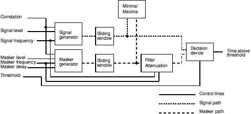
The model calculates a small sample of both masker and signal. The masker and signal can be altered in frequency and also a time delay between the two can be introduced. The envelopes of the masker and signal samples are calculated separately. A sliding window is used to select a number of sequential sections of the masker and signal. A simulated auditory filter is then centred on the signal. The level dependence of the filter is controlled by the instantaneous masker level in the chosen portion. The signal-to-masker ratio at the output of filter is calculated and compared to a criterion ratio. If the signal-to-masker ratio is above the criterion, then that section is counted as providing a detection opportunity in which it is possible for the signal to be detected. The sliding window is advanced throughout the sample and the total number of detection opportunities is calculated, from which the total time in which the signal should be detectable can be derived.
The model is shown in block form in figure 6.1.

Figure 6.1. The detection-time model as a block diagram. The control inputs and signal/masker paths are shown.
Short bursts of signal and masker bands of noise were calculated in a similar way to that used to make the stimuli in previous experiments. The sampling frequency was 16 kHz. For the earlier experiments, a 10 second sample was calculated which could be looped to allow continuous playback (as the bands were composed of sinusoids spaced 0.1 Hz apart). For modelling purposes, only 300 ms was calculated (4800 samples) which was the same as the steady state presentation time of the stimuli in the earlier experiments. For the purposes of the model, only one masking band was calculated which could be placed at any frequency. The masker and signal samples were separately analysed. Firstly, the RMS value of the whole 300ms sample was calculated. Secondly, a sliding window 200 samples in size (12.5 ms) was used. The window size was chosen to be comparable to the equivalent rectangular duration of the temporal window measured by Moore et al. (1988) and Plack and Moore (1990). The window was placed at the start of the whole sample and the RMS value of that 200 sample chunk was calculated. The difference between the RMS value of the windowed chunk and the overall RMS value was calculated. The nominal long-term level of the whole chunk was set prior to running the model; it was therefore possible to calculate the instantaneous level of the sample for that 12.5-ms window. The window was then advanced by 50 samples (3.125 ms) and the instantaneous level re-calculated. The process was repeated until all the 4800 samples had been covered. This gave an approximation to the envelope of the signal. Figure 6.2 shows the technique graphically.
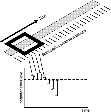
Figure 6.2. A graphical demonstration of the sliding window technique for calculating short-term level.
An example of the envelopes produced by the windowing system is shown in figure 6.3. The samples were not passed through a simulated auditory filter, so the absolute values are not correct.
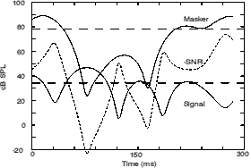
Figure 6.3. An extreme example of what can happen with uncorrelated masker and signal bands. The masker has an overall level of 78 dB SPL (spectrum level 65 dB SPL). The masker and signal level are those used in experiment 3 at threshold. The Noise-to-Signal Ratio (marked as -SNR) goes as low as -20 dB. i.e. the SNR goes as high as +20dB. The horizontal lines represent the long term RMS level of the masker and signal bands. The masker and signal have not passed through a simulated auditory filter.
The envelopes calculated could be passed to one of two other processing mechanisms. One simply calculated the average values of the maxima and minima and also counted the average number of each within the 300ms chunk (the maxima/minima box in figure 6.1). The mechanism for defining a minimum or maximum compared each point to the two adjacent points looking for a turning point (e.g. the centre point has a higher value than the two flanking points for a maximum). The action of this mechanism was instrumental in choosing effective window sizes and the displacement between adjacent window positions. Larger windows would produce much more smoothing and thus it would be possible to miss small turning points. The major part of the model is an auditory filter centred at the signal frequency. The bandwidth of the filter was dependent on the signal frequency and also input level. A rounded exponential filter was used based on the roex(p) filter described by Patterson et al. (1982). The parameter p determines both the bandwidth and the slope of the skirts of the auditory filter. The higher the value of p, the more sharply tuned the filter. The roex(p) filter has only one parameter unlike the roex(p,r) and roex(p,w,t) filters also described by Patterson et al. A smaller number of parameters makes the implementation more simple. The roex(p) filter shape is usually quite successful in predicting the data from notched-noise experiments (which are a common technique for measuring filter shapes). The roex(p) filter becomes a poorer predictor when the thresholds cover a wide range of levels or when the masked thresholds approach the absolute threshold. However, the experiments and model were run using moderate levels and only cases where the masked threshold was well above absolute threshold will be considered in the modelling. Also, the model is to be used in comparisons of conditions. Relative predictions are not altered significantly by filter widths; only the absolute values are altered.
The simulated filter attenuated the masker by a certain amount based on formulae derived by Glasberg and Moore (1990) and Moore and Glasberg (1987). A roex(p) filter shape is given by the following equation (W, g and p are described below):
![]()
![]()
![]()
![]()
![]()
Equation 2 is a mathematical expression of the power-spectrum model. Ps is the power of signal at threshold. N(f) is the long-term power spectrum of the masker. The integral is a simple summation of the masker over all frequencies with W(f) being the weighting applied to the masker at frequency f.
The parameter p determines both the bandwidth and the slope of the skirts of the filter. The higher the value of p, the more sharply tuned is the filter.
It is convenient to measure frequency in terms of the absolute value of the deviation from the centre frequency of the filter, fc, and to normalise this frequency variable by dividing by the centre frequency of the filter. The new frequency variable, g, is defined as:
![]()
![]()
where f = specified frequency and fc = centre frequency.
In terms of the model described here, equation 3 can be written as:
where fm = masker frequency and fs = signal frequency.
![]()
![]()
The attenuation A of the filter at the normalised frequency separation, g, is given by the equation:
![]()
![]()
To allow for an asymmetric filter, the parameter p is allowed to take different values on each side of the filter, i.e. pl and pu. At a level of 51 dB/ERB, pl and pu are roughly equal. Glasberg and Moore (1990) suggested that pu was virtually invariant with level, whereas pl at an input level X (in dB/ERB) is given by the equation:
![]()
![]()
where pl(51) is value of pl at a certain centre frequency for an effective input level of 51 dB/ERB and pl(51,1k) is the value of pl at 1 kHz for an input level of 51 dB/ERB. The term in the first brackets is a correction for values of f that are far from 1 kHz. As the signal was at 1500 Hz, the term was ignored. Thus the equation is simplified to:
![]()
![]()
The ERB of the filter is given by the following equation, where Fs is the CF in kHz:
![]()
![]()
The ERB is related to the value of pl(51) by the equation:
![]()
![]()
In combination, the equations allow us to estimate the level of the masker that passes through the filter depending on the masker level (either long-term or instantaneous level). The signal level is ignored as it is very low compared to the masker level at the input to the filter, and also to simplify the mathematics.
The masker and signal were treated as randomly modulated sinusoids with an instantaneous level corresponding to the output of the sliding window. The masker was reduced in level by the attenuation calculated at the masker frequency (equation 3). The masker level and the signal level could then be compared in each time chunk and if the Signal-to-Noise Ratio (SNR) was greater than a certain threshold value (the detection opportunity threshold, DOT), the signal was taken as providing a detection opportunity in that chunk. The program then summed the time in milliseconds over which it would be possible to detect the signal, i.e. the total detection opportunity time. The concept of having a number of detection opportunities is similar to 'multiple looks' (Viemeister and Wakefield, 1991).
To choose the threshold value (the DOT), the data from experiment 3 were used. The masker level and thresholds measured were used as the masker and signal levels at the input to the model. The correlation between the masker and signal was set appropriately. A range of threshold SNRs was tried. For both the correlated and uncorrelated conditions, 100 samples were calculated and analysed. The results are shown in figure 6.4.
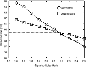
Figure 6.4. The effect of altering the threshold SNR for detection.
The reason for the curves having the form shown in figure 6.4 is discussed later. The crossover point was chosen as the threshold SNR (the DOT) to use for the model. This implies the assumption that the appropriate detection threshold leads to a constant total detection time. The DOT corresponded to a SNR of 2.17 dB. The detection time this corresponded to is 59.5 ms.
The model allowed the filter bandwidth to be dependent upon the input masker level. Figure 6.5 shows the effect of doing this, which is to flatten both curves. The curve for the correlated condition is flattened the most. As the decision device (shown in figure 6.1) is a simple comparator (or all-or-nothing device), then without a level dependence the masker waveform at the output of the simulated filter would be almost the same as the signal waveform at the output of the filter in the correlated condition. In this case, if detection time is plotted against SNR, it will show a step function with the step at 0 dB SNR (figure 6.5 does not take the DOT into account). If the filter bandwidth changes with level this means that the masker waveform is altered somewhat; the masking function then does not have a slope of unity. The more intense sections of the masker waveform cause the filter to broaden more and so they become relatively even more intense at the filter output.
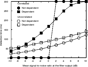
Figure 6.5. The effect of making filter bandwidth dependent upon input level. The signal and maskers level are chosen for illustrative purposes rather than from previous experiments.
The model described here allows the same conditions as used in previous experiments to be applied to it with the limitation that only one masking band is allowed. As experiment 4 showed that the masker band below the signal frequency was responsible for the majority of the masking, the masker frequency applied to the model was always below the signal frequency. When the model was presented with a 65 dB SPL spectrum level masker and with all three masking conditions used in experiment 3 (correlated, uncorrelated and sinusoidal signal), the following output was produced (figure 6.6):
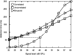
Figure 6.6. Simulating experiment 3 using the detection-time model. Detection times for the actual threshold signal levels are very similar. The dotted lines are discussed in the body of the text.
The choice of the detection opportunity threshold was based on the assumption that detection threshold corresponds to a constant sum of detection opportunities. Is this is a fair assumption? Figure 6.6 illustrates a mapping of signal level to the sum of detection opportunities for three different conditions. If the mean thresholds measured in experiment 3 are used as the signal level, very similar times result (as represented by the dotted lines in figure 6.7). They are especially similar for the conditions used to calibrate the model (i.e. correlated and uncorrelated). The similarity is only to be expected as figure 6.6 was derived by using the thresholds from experiment 3 anyway, but it is reassuring that the mapping between signal level and detection times is commutative.
If one assumes that detectability is monotonically related to the proportion of time that the short-term SNR exceeds the DOT, then the curves produced by the model can be regarded as approximations to psychometric functions or are at least monotonically related to psychometric functions. The model therefore predicts that the psychometric functions for the correlated and uncorrelated conditions should have different slopes. The difference may not be as great as one would think at first glance as the eye is drawn to the intersection of the curves at which point the curve corresponding to the correlated condition is the steepest. The true slopes to compare are the tangents at the points where the threshold signal levels intersect the curves (as shown by the dotted lines). The curves at these points are still very different, but the difference is somewhat smaller than the difference at the intersections of the curves themselves.
Interesting, the model would appear to predict that at high signal levels, a correlated signal should be more detectable than an uncorrelated signal. The reason for the correlated signal having a higher detection time is quite clear; at high signal levels the signal will always be above the masker level in the correlated condition. This is not true for an uncorrelated signal (except for very high signal levels). Figure 6.3 shows the very large variation in instantaneous level of the noise bands. Even if the signal level is high enough so that it should be detectable for a very large majority of the time (e.g. 20 dB above threshold), it is likely that there will be a small number of times in which the signal is not detectable simply because of the large independent variations. Even though the correlated signal has a higher detection time at high SNRs, this does not automatically predict that it should more detectable. The detection time curves are not psychometric functions; they are simply monotonically related to them. This can be shown by considering which portion of the curves the experimentally determined thresholds intersect with. A three-alternative, forced-choice task with a three-down, one-up procedure (as used in all the previous experiments described here) tracks the 79.4% correct point on the psychometric function (Levitt, 1971). The dashed lines in figure 6.6 show that the measured thresholds correspond to the 25-30% region of the detection time function. Therefore only limited parts of the curve may be important and the mapping between detection time and psychometric functions is largely biased to the lower portions of the curve. An example of such a mapping is shown in figure 6.7. The curve was produced with two bezier curves which intersect and the 30/80 point is indicated by the dotted lines. The terminal gradients were constrained to 80/30 at the origin and zero at the (100,100) point.
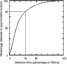
Figure 6.7. A potential mapping between detection time and the psychometric function.
Figure 6.7 shows that for the high detection times (say above 70%) performance is likely to be very close to ceiling and in this region only small differences between the correlated and uncorrelated conditions would be expected. Therefore, it is likely that even if the correlated signal was more detectable at very high signal levels, the effect would not be measurable, due to the ceiling effect.
The prediction of a difference in slopes of the psychometric functions in the region of masked threshold can be tested experimentally. Such an experiment is described next.